Presentation of MTF Simulation of Lenses
Simulation of the performance of photographical lenses
The software MTF Simulation of Lenses perform a simulation of the performance of lenses. In fact, the user select any lens in a data base and a picture. This picture is doe to the simulation modified as the lens will do.
For the simulation the software compute and take in account the following parameters:
Relative -illuminance: this curve indicate the -darkness of the picture on each point of the picture.
The distortion: this curve indicate the distortion on each point of the picture.
The MTF (Modulation Transfer Function) graphs: the MTF graphs indicate the lost of precision on each point of the picture and for each spatial frequency (the measurement unit is the number of lines/mm).
There are 2 kind of MTF diagrams:
MTF tangential
MTF -sagittal
To process a picture, we need to work on a polar coordinates (P,I,J) on the concerned point (P) to process. O is the center of the lens, which is also the center of the negative film.
So OP is the image height (u on Zeiss data sheets). P' is the result of the simulation.
The distortion can be easily calculated with the formula:
![]()
P' is the new point resulted. The distortion is also a locally translation.
The principle of the calculation is to perform an FFT (in 2D) in the polar coordinates, perform an attenuation of the coefficients and perform the inverse FFT.
This FFT produce:
For the
frequency 0, the illumination of the point P (called
![]() )
)
The tangential
spectrum (every frequencies which can be in the form
![]() )
)
The sagittal
spectrum (every frequencies which can be in the form
![]() )
)
So we obtain after processing the FFT the following result:
The computation of the MTF and the relative illuminance consist of multiplicating each Ai,j term through the coefficient of attenuation Mi,j described later:
![]()
The attenuation coefficient Mi,j are:
M0,0: relative illumination on the point P
M0,p: MTF
sagittal on the point P for the frequency
![]() divide
through M0,0.
divide
through M0,0.
Mk,0: MTF
tangential on the point P for the frequency
![]() divide
through M0,0.
divide
through M0,0.
Mk¹0,p¹0: ![]()
To perform the computation, Optical do first the translation caused by the distortion, then apply the calculation of the MTF and the relative illuminance effect.
When MTF Simulation of Lenses is started the following main window will be displayed:

Click on File->Open to load a data base of lenses. A demonstration data base (demo.ldb) is delivered. It contain some data of fictive lenses:
50mm: a fictive lens
filtre_5_raies: a lens which have a MTF equal to 0 on each point for a frequency of 5 lines/mm
filtre_10_raies: a lens which have a MTF equal to 0 on each point for a frequency of 10 lines/mm
transparant: a perfect lens which have a MTF equal to 1 on each point of the picture and for every frequency
filtre_sagital: a lens which have all MTF -sagital equal to 0 on each point and for every frequency
filtre_tangentiel: a lens which have all MTF tangential equal to 0 on each point and for every frequency
Click on Data Base->Visualization to see the characteristic of each lens in the data base:
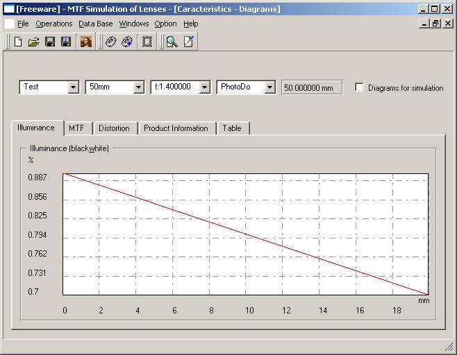
The first line contain the key for choosing the lens:
The manufacturer (here test)
The designation of the lens (here 50 mm)
The aperture (here f1.4)
The source of the measurement (here Photodo)
The -focale (here 50 mm, only as information)
To start the simulation click onto Operation->Simulation on the main window. The following window appear:
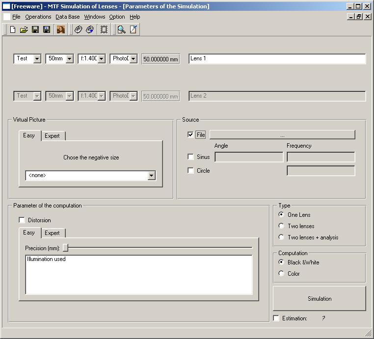
First choose a lens and then a source picture on which the computation will be performed:
File: the source a picture (gif, jpeg, xbm or bmp)
Sinus: the source is a set of line with a frequency of x lines/mm and with an angle of y degree
Circle: the source is a set of circles with x lines/mm centered on the middle point of the lens.
After it, select the output window. This window correspond to the size of the negative.
Attention: Depending on the precision and the size of the window, the quantity of the memory request and the computation time can be very important. (for a whole 32mm negative with a precision of 40 lines/mm, the computation can take a half day for a Pentiun 4)
The last operation is the selection of the precision. It is possible to modify it directly (using the text entry) or using the slider. If the distortion should be calculated the field distortion must be selected.
Now, click on simulate to start the simulation.
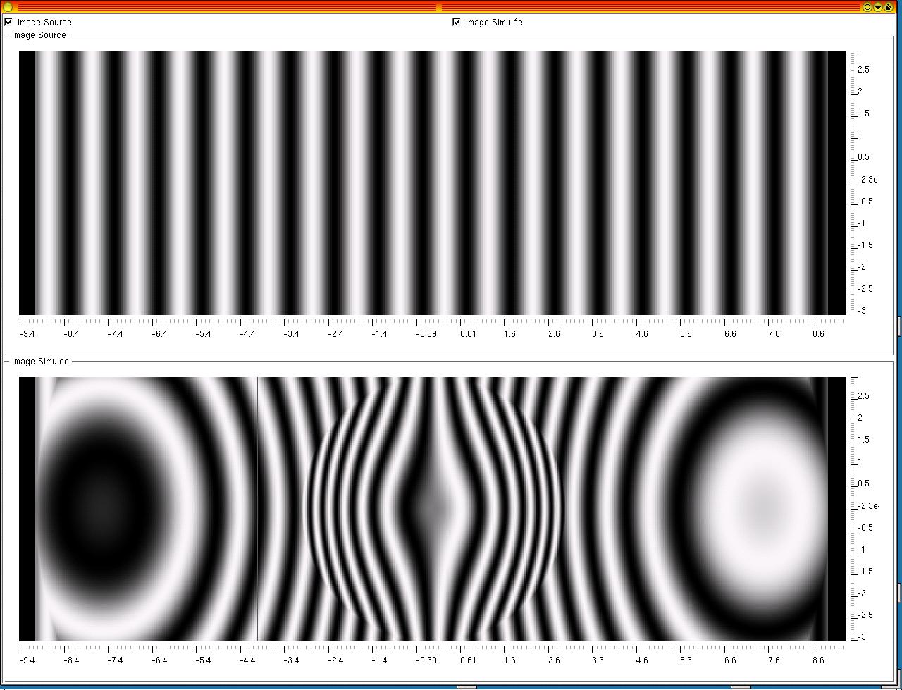
After the computation, the result appear on a new window which permit to compare the simulated picture with the source picture:
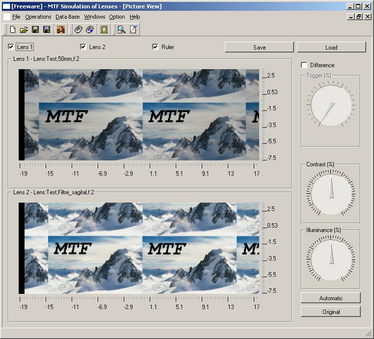
It is possible to zoom in/out the simulated and the original picture by selecting an area with the mouse.
This is the result of the simulation of a lens with a distortion which go from +100% to -100%.
This example is the simulation of a lens which have a MTF equal to 0 for 5 lines/mm. The source picture is composed from lines with a frequency of 5 lines/mm. The result is a picture grey.

This example is the simulation of a lens which have a MTF sagital equal to 0 for 5 lines/mm. The source picture is composed from lines with a frequency of 5 lines/mm. The lens filter all lines which are going through the center of the lens.
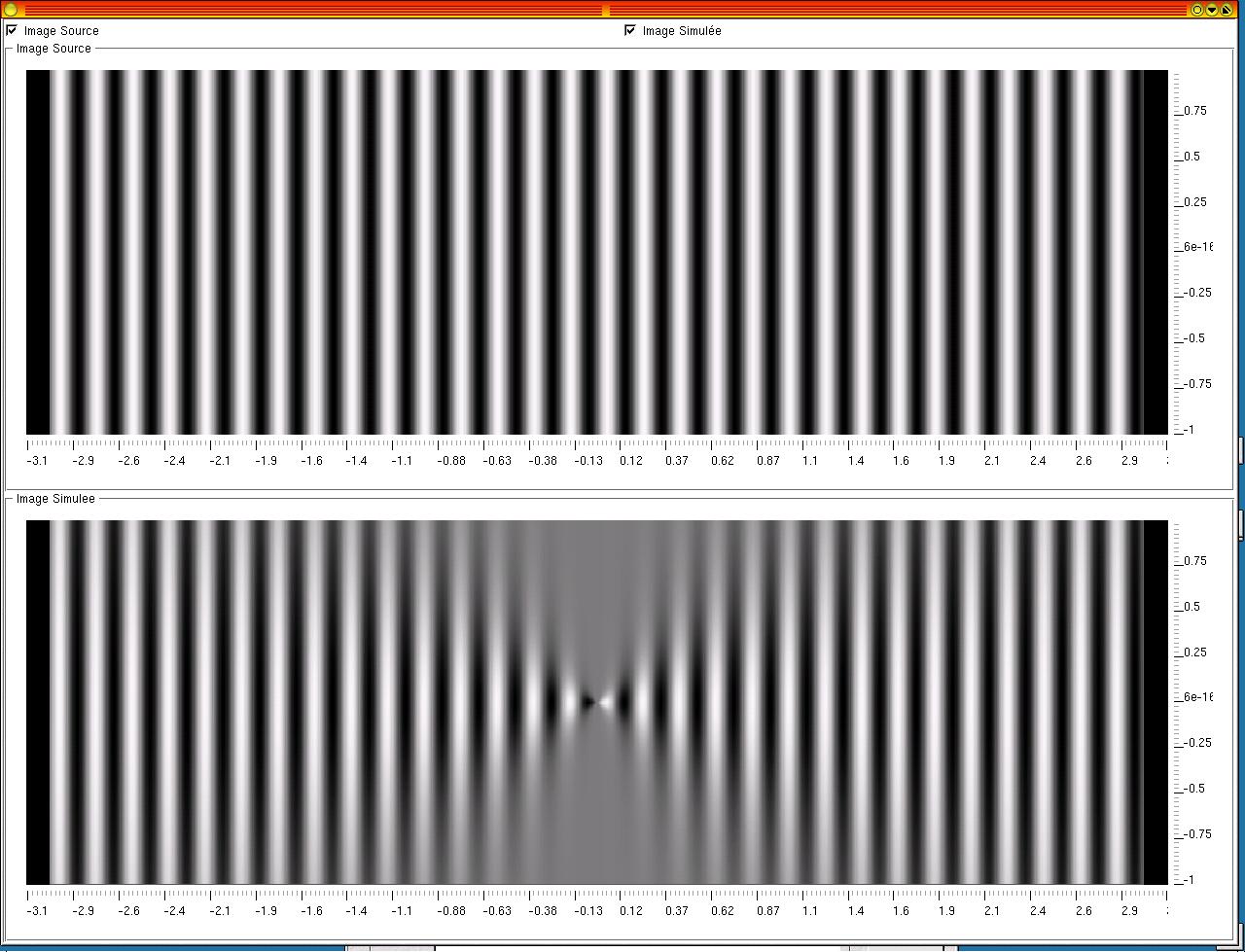
This example is the simulation of a lens which have a MTF tangential equal to 0 for 5 lines/mm. The source picture is composed from lines with a frequency of 5 lines/mm. The lens filter all lines which are tangential to a circle centered on the center of the lens.

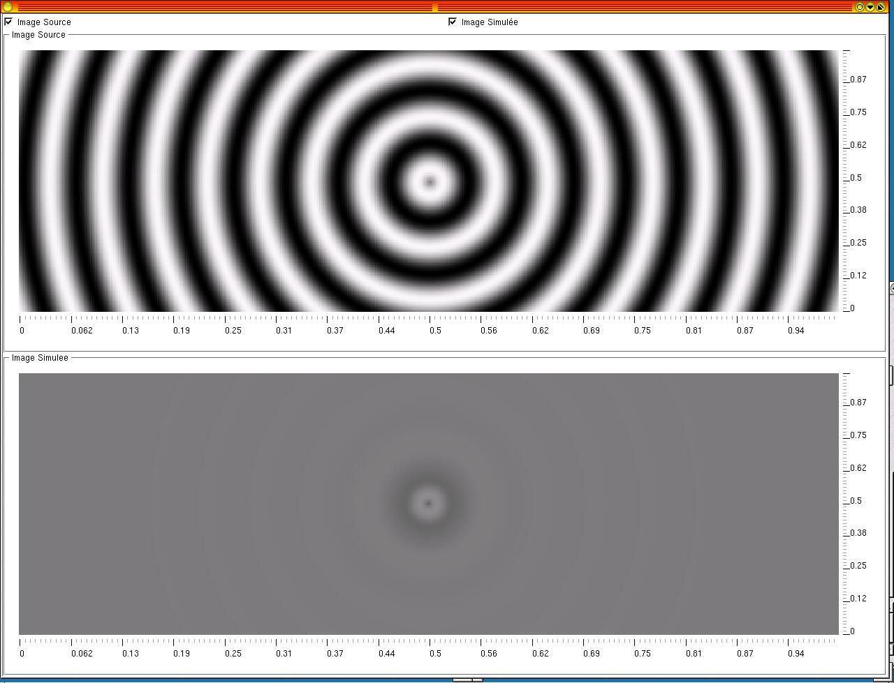
When the source picture contain only some circles with a spatial frequency of 5 lines/mm , the result is a picture fully gray.
Author: Sebastien Fricker
E-Mail: friseb123@users.sourceforge.net